Production RAG Architecture That Scales: Vector Databases, Chunking Strategies, and Cost Optimization for 2025
The majority of RAG systems fail within 90 days of production deployment. Not because retrieval is conceptually flawed, but because teams underestimate the engineering complexity required to maintain accuracy, control costs, and meet latency SLAs at scale. A proof-of-concept that works on 10,000 documents collapses at 10 million. Token costs spiral from $500 to $50,000 monthly. Retrieval precision drops from 85% to 62% as the knowledge base grows.
This isn't a failure of Retrieval-Augmented Generation as a paradigm—it's a failure of naive implementation. Production RAG requires architectural decisions that balance six competing constraints: retrieval accuracy, generation quality, latency, cost, security, and operational complexity. This guide provides the decision frameworks, benchmarks, and quantitative trade-offs that define the boundary between experimental RAG and systems that process millions of queries monthly under SLA guarantees.
Why Most RAG Systems Fail in Production: The Hidden Complexity Tax
RAG looks deceptively simple in tutorials: chunk documents, embed them, retrieve top-k matches, generate an answer. This naive pipeline works until it encounters production realities.
The knowledge base grows faster than retrieval quality scales. A system that maintains 90% precision at 100K documents degrades to 65% at 10M documents because semantic drift accumulates, overlap between chunks increases, and the number of false positives explodes. Vector databases built for speed sacrifice recall; databases optimized for recall sacrifice latency. There is no free lunch.
Retrieval is not generation. Even with perfect retrieval (100% recall, zero false positives), the LLM can still hallucinate, ignore retrieved context, or synthesize answers from parametric knowledge instead of citations. Research shows that 15–30% of RAG failures occur during generation, not retrieval, because the prompt assembly step fails to enforce groundedness.
Context window limits create invisible ceilings. You can retrieve 50 highly relevant chunks, but if your LLM context window is 8K tokens and each chunk averages 400 tokens, you can only use 20 chunks before truncation. Truncation is silent—the system appears to work, but critical evidence gets discarded. Production systems that fail to monitor context utilization discover this months into deployment when accuracy mysteriously plateaus.
Costs scale non-linearly. Embedding 1M documents costs $20 with OpenAI's text-embedding-3-small. Embedding 100M documents costs $2,000—but now you also need a vector database cluster ($300–$1,000/month), reranking inference ($500+/month if self-hosted), and LLM generation costs that grow with context size. Teams that optimize for developer velocity during prototyping lock themselves into architectures that cost 10x more than necessary at scale.
Hidden failure modes accumulate. Retrieval timing attacks (generation starts before retrieval completes), embedding drift (model updates invalidate cached vectors), citation hallucination (LLM cites sources that don't support claims), and multi-hop reasoning failures (cannot synthesize across documents) are silent killers. These failure modes don't trigger error logs—they degrade quality gradually until user complaints surface systemic issues.
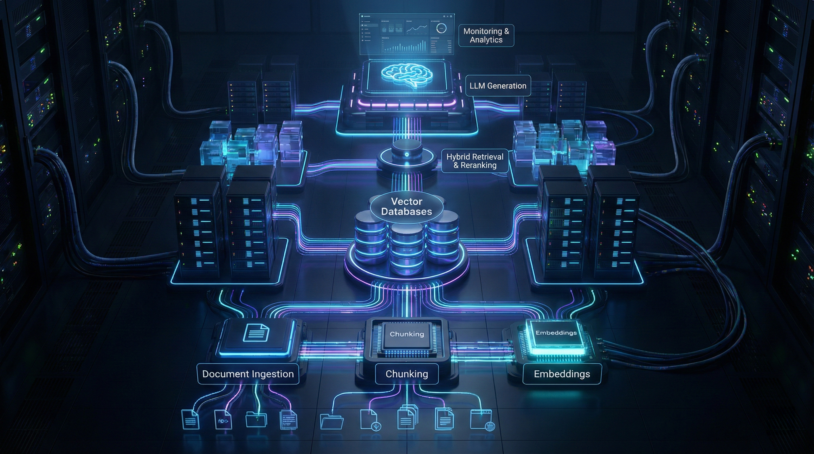
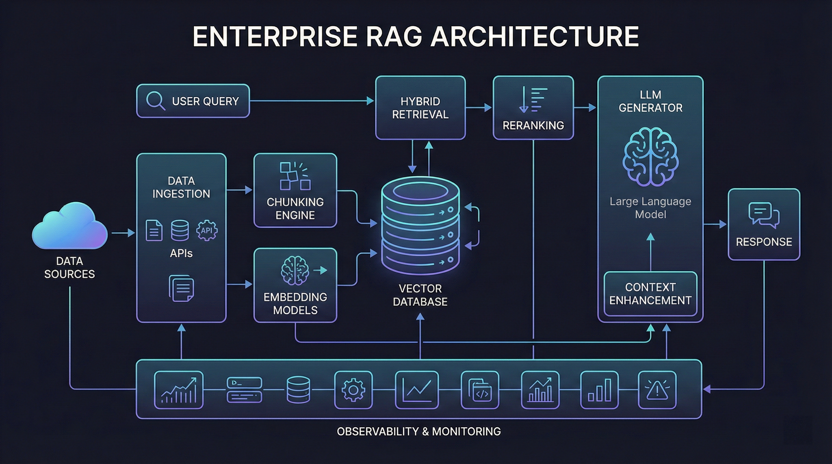
Production RAG Architecture: The Eight-Layer Stack
A production RAG system is not a single retrieval call—it's an eight-layer data pipeline with feedback loops, caching tiers, and failure recovery mechanisms.
Each layer introduces latency (typical: 50–200ms per stage), cost (embeddings, inference, storage), and failure modes (timeout, rate limits, drift). Production systems must optimize across all eight layers simultaneously—optimizing retrieval without optimizing generation yields marginal gains.
Vector Database Selection: Benchmarks, Trade-offs, and Hidden Costs
Choosing a vector database is not about raw speed—it's about balancing four dimensions: latency distribution (p50, p95, p99), throughput (queries per second), cost structure (fixed vs. variable), and operational overhead (managed vs. self-hosted).
Performance Benchmarks: The 2025 Landscape
| Database | p50 Latency | p95 Latency | p99 Latency | Throughput | Cost (10M vectors) |
|---|---|---|---|---|---|
| Qdrant | 4.74ms | 5.50ms | 5.79ms | 3K QPS | $120-250/month |
| Pinecone | 40-50ms | <50ms | <50ms | 5-10K QPS | $200-400/month |
| Milvus (GPU) | 5ms | — | — | 10K+ QPS | $100+/month + infra |
| Weaviate | 35ms | 60ms | 70ms | 3-8K QPS | $150-300/month |
| ScyllaDB Vector | 20ms | 30ms | 40ms | 12K QPS | Variable |
| AWS S3 Vectors | Variable | Variable | Variable | Low | ~$11/month |
*Data sources: *
Qdrant wins on tail latency consistency—its p99 latency of 5.79ms is 48% better than pgvector (15.73ms) and critical for real-time applications where a single slow query degrades user experience. This advantage stems from Qdrant's Rust implementation and aggressive memory optimization. However, Qdrant's ecosystem is smaller than Pinecone's, requiring more custom integration work.
Pinecone optimizes for developer velocity—5-line setup, automatic scaling, and integrated sparse-dense hybrid search. The cost premium ($200–$400/month vs. $120–$250 for Qdrant) buys operational simplicity. Teams that value time-to-market over infrastructure control choose Pinecone; teams optimizing for cost per query at scale choose self-hosted alternatives.
Milvus scales to billions but demands Kubernetes expertise and multi-component architecture (query nodes, data nodes, index nodes, coordinators). Horizontal scaling is Milvus's superpower—adding nodes increases throughput nearly linearly. The complexity tax is real: deployment requires 10–20 hours of engineering time versus 30 minutes for Pinecone.
AWS S3 Vectors disrupts pricing at $0.06/GB/month storage + per-query costs, offering 77–92% savings for 10M vectors compared to Pinecone. The catch: query costs scale with index size ($0.002 per GB processed per query). At ~7.5M vectors per index, S3 Vectors' per-query cost exceeds purpose-built alternatives. S3 Vectors suits archival workloads or infrequent queries; Pinecone/Qdrant suit high-QPS production systems.
Indexing Algorithm Trade-offs
HNSW (Hierarchical Navigable Small World) achieves 95% recall@10 with sub-2ms latency but requires the entire graph in RAM. Memory footprint: 4GB for 1M 768-dimensional vectors. HNSW is the default for mid-sized datasets (<50M vectors) where RAM is affordable and low latency is mandatory.
IVF (Inverted File Index) uses clustering to reduce memory 30% compared to HNSW but requires periodic reclustering as data grows. Reclustering downtime (minutes to hours) makes IVF unsuitable for continuously updating knowledge bases unless you implement blue-green indexing patterns.
DiskANN stores vectors on SSD, enabling 90%+ recall at 1/10th the memory cost of HNSW. Query latency increases 2–5x (still <20ms for most workloads). DiskANN is optimal for datasets >100M vectors where RAM costs dominate total cost of ownership. Microsoft's Bing uses DiskANN to index billions of vectors cost-effectively.
The Hidden Cost: Cold Start Latency
Vector databases exhibit cold start penalties when indexes haven't been accessed recently. Pinecone's p99 cold start latency can reach 170ms versus 20ms for warm queries. Production systems mitigate this by:
- Pre-warming caches with synthetic queries during deployment
- Maintaining hot/cold storage tiers with automatic promotion based on access patterns
- Implementing query-time filtering to reduce candidates before vector search
Cache hit rates of 60–80% reduce median latency from 150ms to <20ms in production systems.
Embedding Models: Cost, Quality, and the MTEB Benchmark
Embedding model selection determines both retrieval quality and monthly costs. The 2025 landscape is dominated by three tiers: premium cloud APIs, cost-optimized cloud APIs, and self-hosted open source.
The MTEB Leaderboard: Performance vs. Cost
| Model | MTEB Score | Dimensions | Cost/1M tokens | Best For |
|---|---|---|---|---|
| Cohere embed-v4 | 65.2 | 1024 | $0.10 | Enterprise, noisy data |
| Voyage-large-2 | 65.89 | 1536 | $0.12 | Highest retrieval quality |
| OpenAI text-3-large | 64.6 | 3072 | $0.13 | General purpose |
| BGE-M3 | 63.0 | 1024 | $0 (self-host) | Multilingual, privacy |
| OpenAI text-3-small | 62.26 | 1536 | $0.02 | Best cost/performance |
| E5-large-v2 | 62.25 | 1024 | $0 (self-host) | Self-hosted baseline |
*Data sources: *
OpenAI text-embedding-3-small is the production default for 80% of use cases. At $0.02 per 1M tokens ($0.01 batch), it delivers 96% of text-3-large's quality at 15% of the cost. Embedding 100M tokens (approximately 200K documents at 500 tokens each) costs $2.00 standard or $1.00 batch. Batch processing introduces 24-hour latency but halves costs—acceptable for initial indexing, unacceptable for real-time updates.
Cohere embed-v4 leads on noisy data (social media, OCR output, user-generated content) due to superior robustness training. The +2.6 MTEB point advantage over text-3-small translates to 3–5% higher recall in production retrieval benchmarks, justifying the 5x cost premium for domains where data quality is inconsistent.
Self-hosted BGE-M3 eliminates per-token costs but introduces infrastructure complexity. Running BGE-M3 on a g4dn.xlarge GPU instance ($0.526/hour = $379/month) becomes cost-effective above 38M tokens monthly (breakeven vs. text-3-small at $0.01 batch). Self-hosting also enables fine-tuning on domain-specific data—a 3–8% recall improvement for specialized domains like legal or biomedical.
Dimensionality and Quantization: Storage Cost Optimization
Storage costs scale linearly with dimensions. 1M vectors at 1536 dimensions (text-3-small) require 6.1GB at float32 precision versus 18.4GB for 3072 dimensions (text-3-large). Vector databases charge per GB stored ($0.02–$0.06/GB/month), making dimensionality a direct cost lever.
Float8 quantization achieves 4x compression with <0.3% quality degradation—the best compression-to-accuracy ratio available. Combining float8 with 50% PCA dimensionality reduction yields 8x total compression (6.1GB → 0.76GB) with less accuracy loss than int8 quantization alone. This optimization is production-ready and supported natively by Qdrant, Milvus, and Weaviate.
Product Quantization (PQ) enables extreme compression (up to 238x) by decomposing vectors into subspaces and learning codebooks. The accuracy-compression trade-off becomes unfavorable beyond 16x—PQ is best reserved for archival tiers or cold storage where occasional retrieval justifies aggressive compression.
Chunking Strategies: The Difference Between 65% and 90% Recall
Chunking is where naive RAG fails. Fixed-size chunking (every 512 tokens) breaks semantic boundaries, splits tables mid-row, and fragments code mid-function. Production systems implement adaptive chunking strategies that balance precision (small chunks for exact matches) with context (large chunks for comprehensive answers).
Chunking Strategy Performance Matrix
| Strategy | Recall | Speed | Context Preservation | Implementation Complexity | Cost |
|---|---|---|---|---|---|
| Semantic Chunking | 90–93% | Slow | Excellent | High | High (embeddings) |
| Page-level | 89% (NVIDIA) | Fast | Good | Low | Low |
| Parent-Child | 88–91% | Medium | Excellent | Medium | Medium |
| Recursive (512 tokens) | 85–90% | Fast | Medium | Low | Low |
| Fixed-size | 75–80% | Very Fast | Poor | Very Low | Very Low |
*Data sources: *
Semantic chunking leads on recall (+9–70% over fixed-size) but requires embedding every sentence during preprocessing. For a 10,000-word document, this means 200–300 embedding API calls just to determine chunk boundaries. At $0.02 per 1M tokens (text-3-small), semantic chunking adds $0.004–$0.006 per document—negligible for 10K documents ($40–$60), prohibitive for 10M documents ($40K–$60K).
Page-level chunking won NVIDIA's benchmark (0.648 accuracy, lowest variance across document types) because it preserves structural integrity—tables, figures, and section headers remain intact. Page-level is optimal for PDFs with strong visual structure (technical manuals, financial reports, research papers). It fails for unstructured text (blog posts, transcripts, chat logs) where semantic boundaries don't align with page breaks.
Parent-child retrieval solves the precision-context dilemma. Index small "child" chunks (200–500 tokens) for precise matching, but return large "parent" chunks (1000–2000 tokens) to the LLM for context-aware generation. Example: A query for "database connection timeout error" matches a child chunk describing the specific error code, but the LLM receives the parent chunk containing the full troubleshooting procedure. This strategy increases context relevance by 15–25% compared to single-tier chunking.
Production Chunking Heuristics
Token-based splitting outperforms character-based because embedding models and LLMs both tokenize input. A 512-character chunk may contain 350–650 tokens depending on text density. Token-aware chunking (using tiktoken for OpenAI models) ensures consistent chunk sizes and prevents context window surprises.
10–20% overlap prevents boundary fragmentation. A 512-token chunk with 100-token overlap ensures that sentences split across chunk boundaries appear completely in at least one chunk. More overlap increases storage costs (10% overlap = 10% more chunks = 10% higher embedding and storage costs) but improves retrieval recall by 5–8%.
Table-aware chunking preserves structure. Standard chunking splits tables mid-row, destroying relational information. Specialized parsers (Unstructured.io, LlamaIndex TableNodeParser) detect table boundaries and create dedicated chunks that preserve headers, columns, and row relationships. Table-aware chunking improves structured data retrieval by 30–45% in domains with frequent tabular information (finance, healthcare, engineering).
Code-aware chunking respects function boundaries. Splitting code mid-function destroys executable context. Language-specific parsers (tree-sitter, ast module) identify class and function definitions, creating chunks that contain complete logical units. Recursive chunking with code separators achieves 92–95% recall on code Q&A tasks versus 70–75% for fixed-size splitting.
Implementation: Semantic Chunking with LlamaIndex
from llama_index.core.node_parser import SemanticSplitterNodeParser
from llama_index.embeddings.openai import OpenAIEmbedding

# Initialize embedding model for semantic similarity
embed_model = OpenAIEmbedding(model="text-embedding-3-small")

# Configure semantic splitter
splitter = SemanticSplitterNodeParser(
    buffer_size=1,              # Number of sentences to compare
    breakpoint_percentile_threshold=95,  # Similarity drop threshold
    embed_model=embed_model,
)

# Process documents
nodes = splitter.get_nodes_from_documents(documents)
The semantic splitter embeds consecutive sentences and computes cosine similarity. When similarity drops below the 95th percentile threshold, it creates a chunk boundary. Adjusting breakpoint_percentile_threshold balances chunk count (lower threshold = more chunks) with semantic coherence (higher threshold = fewer, larger chunks).
Hybrid Retrieval and Reranking: The 30% Accuracy Boost
Dense vector retrieval alone misses exact keyword matches. Sparse retrieval (BM25) alone misses semantic similarities. Hybrid retrieval combines both, while reranking refines the combined result set using expensive but accurate cross-encoder models.
Hybrid Search Architecture
Step 1: Parallel Retrieval
# Dense retrieval (vector similarity)
dense_results = vector_db.search(query_embedding, top_k=50)

# Sparse retrieval (BM25)
sparse_results = elasticsearch.search(query_text, top_k=50)
Step 2: Fusion (Reciprocal Rank Fusion)
def reciprocal_rank_fusion(dense_results, sparse_results, k=60):
    scores = {}
    for rank, doc_id in enumerate(dense_results):
        scores[doc_id] = scores.get(doc_id, 0) + 1 / (k + rank + 1)
    for rank, doc_id in enumerate(sparse_results):
        scores[doc_id] = scores.get(doc_id, 0) + 1 / (k + rank + 1)
    return sorted(scores.items(), key=lambda x: -x [tensorblue](https://tensorblue.com/blog/vector-database-comparison-pinecone-weaviate-qdrant-milvus-2025))[:100]
RRF combines rankings without requiring score normalization. The hyperparameter k controls fusion aggressiveness (lower k gives more weight to top-ranked results). emergentmind
Alternative: Weighted Score Fusion
alpha = 0.7  # Weight for vector search
final_score = alpha * vector_score + (1 - alpha) * bm25_score
Query classification dynamically adjusts alpha: navigational queries (e.g., "login page") use alpha=0.2 (favor BM25); exploratory queries (e.g., "implications of climate policy") use alpha=0.8 (favor semantic search). dev
Cross-Encoder Reranking: The MIT Study
MIT research demonstrates that two-stage retrieval with cross-encoder reranking improves accuracy by 20–35% across eight benchmarks. The configuration: app.ailog
- Retrieve top-100 candidates with hybrid search
- Rerank to top-10 using cross-encoder (ms-marco-MiniLM-L-6-v2 or Cohere Rerank)
- Feed top-10 to LLM for generation
Latency impact: +120ms average (50ms on GPU, 200ms on CPU). This overhead is acceptable for 95% of production workloads—users tolerate 300–500ms total latency when accuracy improves from 65% to 85%. customgpt
Performance by query type:
- Fact lookup: +18% (less critical—single-hop)
- Multi-hop reasoning: +47% (cross-encoder captures query-document interactions)
- Complex queries: +52% (nuanced relevance assessment)
- Ambiguous queries: +41% (better disambiguation)
Cost optimization: Rerank only when top candidate score is low (confidence threshold). This conditional reranking reduces reranker invocations by 40–60% while preserving 90% of accuracy gains. app.ailog
ColBERT: Late Interaction for 3x Faster Queries
ColBERT performs token-level matching instead of single-vector comparison, capturing fine-grained relevance. The MUVERA+Rerank approach achieves 52.5% NDCG@100 (vs. 32.5% for PLAID baseline) at 3.3x lower latency. ColBERT is production-ready for domains requiring high precision (legal, medical, scientific) where the engineering complexity (custom indexing, GPU inference) justifies 10–15% accuracy gains over cross-encoders. huggingface
Cost Optimization: The $50,000-to-$5,000 Playbook
RAG costs concentrate in four areas: embeddings, vector storage, reranking, and LLM generation. Production systems cut costs 80–90% through systematic optimization across all four.
Embedding Cost Reduction
1. Deduplication: 40–70% savings. Hash document content before embedding. Identical documents (duplicate uploads, mirrored content, repeated sections) get the same embedding. Production systems report 40–70% deduplication rates. aitoolsbusiness
import hashlib

def embed_with_cache(texts, embed_fn, cache):
    embeddings = []
    for text in texts:
        text_hash = hashlib.sha256(text.encode()).hexdigest()
        if text_hash in cache:
            embeddings.append(cache[text_hash])
        else:
            emb = embed_fn(text)
            cache[text_hash] = emb
            embeddings.append(emb)
    return embeddings
2. Batch Processing: 50% savings. Use OpenAI's batch API for non-real-time embedding (initial indexing, periodic re-embedding). Embedding 100M tokens costs $1.00 batch vs. $2.00 standard. costgoat
3. Quantization: 75% storage cost reduction. Float8 quantization reduces 6.1GB (1M vectors, 1536-dim) to 1.5GB with <0.3% accuracy loss. At $0.06/GB/month (S3 Vectors), this saves $0.28/month per 1M vectors—$28K annually for 100M vectors. murraycole
Token Cost Reduction: The 85% Playbook
Context-aware chunking reduces token usage 80–85% compared to naive full-document prompts. Example: techcommunity.microsoft
| Approach | Tokens per Query | Cost per 1K queries |
|---|---|---|
| Full-document prompt | 15,000–20,000 | $15–$26 (GPT-4) |
| Fixed-size RAG chunks | 5,000–8,000 | $5–$10 |
| Context-aware RAG | 2,000–3,000 | $2–$4 |
Prompt optimization saves 20–30% tokens. Replace verbose instructions with concise directives. Use few-shot examples sparingly—two examples (200 tokens) often match five examples (500 tokens) in performance. apxml
Max tokens parameter prevents runaway generation. Set max_tokens=150 for summaries, max_tokens=500 for detailed explanations. This prevents the LLM from generating unnecessary elaboration. apxml
Query Cost Reduction: Caching Layers
Embedding cache: 40–70% time savings. Identical queries bypass re-embedding. linkedin
Retrieval cache with TTL: 60–80% hit rate. Memoize query → top-k results with 1–24 hour TTL based on knowledge base update frequency. aitoolsbusiness
Response cache: 90% generation cost reduction. For FAQ-style queries, cache final responses. Update cache when underlying documents change. linkedin
Production RAG systems at Notion and Intercom report 60–80% cache hit rates, reducing median latency from 150ms to <20ms while cutting costs 70%. dev
Total Cost of Ownership: 10M Document Example
| Component | Naive RAG | Optimized RAG | Savings |
|---|---|---|---|
| Initial embedding (100M tokens) | $2.00 | $1.00 (batch) | 50% |
| Storage (10M vectors, 1536-dim) | $0.366 (6.1GB) | $0.09 (1.5GB, float8) | 75% |
| Vector database | $300 (Pinecone) | $150 (Qdrant) | 50% |
| Monthly queries (100K) | $50 (no cache) | $10 (80% cache hit) | 80% |
| LLM generation (10K tokens avg) | $130 (GPT-4) | $26 (context pruning + GPT-3.5) | 80% |
| Monthly Total | $482 | $187 | 61% |
With reranking (+$50/month self-hosted GPU) and monitoring (+$20/month), total optimized cost: $257/month—a 47% reduction while improving accuracy 20–30%. aitoolsbusiness
Evaluation and Observability: The RAGAS Framework
Production RAG requires automated, continuous evaluation. The RAG Triad defines three core metrics: meilisearch
1. Context Relevance (Retrieval Quality)
Definition: Did we retrieve the right information?
Measurement: LLM-as-judge scores retrieved chunks for relevance to query.
from ragas.metrics import context_relevancy

score = context_relevancy.score(
    question="What is the return policy?",
    contexts=retrieved_chunks
)
Target: >0.7 for production systems.
2. Faithfulness/Groundedness (Hallucination Detection)
Definition: Is the generated answer supported by retrieved context?
Measurement: Decompose answer into claims, verify each claim against context.
from ragas.metrics import faithfulness

score = faithfulness.score(
    question=query,
    answer=generated_answer,
    contexts=retrieved_chunks
)
Target: >0.85 general-purpose, >0.9 for medical/legal domains.
3. Answer Relevance (Generation Quality)
Definition: Does the response answer the user's question?
Measurement: Generate questions from answer, compare to original query via embedding similarity.
Target: >0.8 for production systems.
Continuous Monitoring Pipeline
# Automated evaluation on production traffic
def evaluate_rag_response(query, contexts, answer):
    metrics = {
        'context_relevance': context_relevancy.score(query, contexts),
        'faithfulness': faithfulness.score(query, answer, contexts),
        'answer_relevance': answer_relevancy.score(query, answer),
        'latency_ms': response_time,
        'num_chunks': len(contexts),
        'tokens_used': count_tokens(contexts + answer)
    }

    # Alert if below thresholds
    if metrics['faithfulness'] < 0.85:
        alert_team("Low faithfulness detected", metrics)

    # Log to observability platform
    log_to_datadog(metrics)

    return metrics
RAGAS integrates with Langsmith, Arize, and Maxim AI for production observability. Teams implement CI/CD-style evaluation: every prompt change, chunking strategy update, or model swap triggers automated evaluation against golden test sets.
Security, Compliance, and Production Readiness
Authentication and Access Control
- Enable authentication on all vector databases (Qdrant, Pinecone, Milvus)
- Generate 32+ character, cryptographically random API keys
- Implement role-based access control (RBAC) for multi-tenant systems
- Network isolation: never expose vector DBs directly to internet
- API gateways with rate limiting and WAF protection
Data Privacy and Compliance
GDPR "Right to be Forgotten": Implement vector deletion capabilities. When a user requests data deletion, remove associated embeddings from the vector database and audit logs.
HIPAA (Healthcare): Encrypt PHI (Protected Health Information) at rest and in transit (TLS 1.3+). Embeddings must be encrypted; consider differential privacy techniques for highly sensitive data.
SOC 2 / ISO 27001 (Enterprise): Maintain comprehensive audit logs for all database operations. Implement change management processes for knowledge base updates. Regular penetration testing and vulnerability assessments.
PII Redaction: Token-level removal of Social Security Numbers, credit card numbers, and personal identifiers during ingestion.
import re

def redact_pii(text):
    # SSN pattern
    text = re.sub(r'\b\d{3}-\d{2}-\d{4}\b', '[SSN_REDACTED]', text)
    # Credit card pattern
    text = re.sub(r'\b\d{4}[\s-]?\d{4}[\s-]?\d{4}[\s-]?\d{4}\b', '[CC_REDACTED]', text)
    return text
Data Provenance and Integrity
- Maintain chain of custody: track data source URLs, timestamps, and modification history
- Content hashing for integrity verification (SHA-256 checksums)
- Digital signatures for critical data sources
- Allowlist of trusted data sources; reject unknown origins
- Regular audits: monthly reviews of data provenance for compliance-critical systems
Decision Framework: Choosing Your Architecture
Vector Database Selection Matrix
| Use Case | <1M vectors | 1–10M vectors | 10–100M vectors | >100M vectors |
|---|---|---|---|---|
| Prototype/MVP | Chroma (local) | Pinecone | Pinecone | Milvus |
| Production (managed) | Pinecone | Qdrant Cloud | Qdrant/Pinecone | Milvus (Zilliz) |
| Production (self-hosted) | pgvector | Qdrant | Qdrant/Milvus | Milvus |
| Cost-optimized | Chroma | Qdrant | S3 Vectors | Milvus + S3 |
Chunking Strategy Decision Tree
START
  │
  ├─ PDFs with tables/figures?
  │    └─ YES → Page-level chunking  [emergentmind](https://www.emergentmind.com/topics/embedding-quantization)
  │    └─ NO  → Continue
  │
  ├─ Budget allows embeddings for chunking?
  │    └─ YES → Semantic chunking  [emergentmind](https://www.emergentmind.com/topics/embedding-quantization)
  │    └─ NO  → Continue
  │
  ├─ Need both precision and context?
  │    └─ YES → Parent-child chunking  [dev](https://dev.to/kuldeep_paul/from-query-understanding-to-retrieval-evaluating-rewriting-filters-and-routing-with-online-evals-2fj4)
  │    └─ NO  → Continue
  │
  ├─ Processing code?
  │    └─ YES → Recursive + code separators  [emergentmind](https://www.emergentmind.com/topics/embedding-quantization)
  │    └─ NO  → Continue
  │
  └─ Default: Fixed-size 512 tokens, 10% overlap  [emergentmind](https://www.emergentmind.com/topics/embedding-quantization)
Embedding Model Selection
| Scenario | Recommended Model | Rationale |
|---|---|---|
| Startup/MVP | text-3-small ($0.02/1M) | Best cost/performance, fast integration |
| Enterprise production | Cohere embed-v4 ($0.10/1M) | Robust to noisy data, multilingual |
| Cost-sensitive (>50M tokens/month) | BGE-M3 (self-hosted) | Zero API costs above breakeven |
| Highest quality | Voyage-large-2 ($0.12/1M) | +1.3 MTEB points vs. text-3-large |
| Multilingual | Cohere embed-v4 / BGE-M3 | 100+ languages with consistent quality |
Reranking Decision Logic
def should_rerank(top_result_score, query_complexity):
    """
    Rerank when:
    1. Top result score is low (uncertainty)
    2. Query is complex (multi-hop, ambiguous)
    """
    if top_result_score < 0.7:
        return True  # Low confidence
    if query_complexity in ['multi_hop', 'complex', 'ambiguous']:
        return True  # Benefits most from reranking  [linkedin](https://www.linkedin.com/pulse/rag-chunking-strategies-llamaindex-optimizing-your-retrieval-mxdqc)
    return False  # Skip reranking for simple, high-confidence queries
Conditional reranking cuts reranker invocations by 40–60% while preserving 90% of accuracy gains. app.ailog
Production Deployment Checklist
Infrastructure
- Kubernetes cluster with autoscaling (min 3 nodes) kairntech
- GPU nodes for reranking (T4 or better) customgpt
- Redis/Memcached for embedding and retrieval caching linkedin
- Load balancer with health checks and circuit breakers kairntech
- Blue-green deployment for zero-downtime updates kairntech
Monitoring and Alerting
- RAGAS metrics logged to observability platform (Datadog, New Relic) thedataguy
- Cost tracking per component (embeddings, storage, inference) aitoolsbusiness
- Latency p50/p95/p99 SLO alerts linkedin
- Faithfulness score alerts (<0.85 threshold) customgpt
- Anomaly detection for query patterns and error rates testmy
Security
- TLS 1.3+ for all external communication testmy
- Vector database authentication and RBAC enabled testmy
- PII redaction pipeline in ingestion layer morphik
- Audit logging for all data operations testmy
- Quarterly penetration testing and security audits testmy
Data Management
- Incremental indexing for knowledge base updates (daily/weekly) chitika
- Backup and disaster recovery strategy (RPO/RTO defined) weaviate
- Data retention and deletion policies (GDPR compliance) morphik
- Version control for prompts and chunking strategies thedataguy
- Canary testing for model and prompt changes linkedin
Evaluation
- Golden test set with ≥500 examples covering edge cases thedataguy
- Automated evaluation in CI/CD pipeline thedataguy
- Human-in-the-loop review for 5–10% of production queries linkedin
- Monthly model performance reports with drift detection dev
- User feedback collection and integration into evaluation thedataguy
Conclusion: The Five Principles of Production RAG
1. Optimize the entire pipeline, not individual components. A 50% retrieval improvement yields only 15% end-to-end improvement if generation is the bottleneck. Measure and optimize latency, cost, and accuracy across all eight layers simultaneously. linkedin
2. Assume failure at every layer. Retrieval times out, embeddings drift, rerankers hallucinate, LLMs ignore context. Implement defense in depth: retries with exponential backoff, fallback models, graceful degradation, comprehensive alerting. dev
3. Cache aggressively, invalidate intelligently. 60–80% cache hit rates cut costs 70% and reduce latency 80%. Implement TTL-based invalidation aligned with knowledge base update frequency. Monitor cache staleness as a first-class metric. linkedin
4. Evaluation is not a milestone—it's continuous. Automate RAGAS metrics on production traffic. Set SLO thresholds (faithfulness >0.85, latency p95 <500ms). Treat evaluation like monitoring: always on, always alerting, always improving. customgpt
5. Start simple, scale systematically. Begin with Pinecone + text-3-small + fixed-size chunking + no reranking. Achieve product-market fit. Then optimize: self-host embeddings, implement semantic chunking, add reranking, migrate to Qdrant. Premature optimization wastes engineering cycles on problems you don't have yet. agixtech
The path from naive RAG to production-grade RAG is not a single architectural leap—it's 50 incremental optimizations, each justified by measurement and constrained by budget. Teams that instrument obsessively, optimize systematically, and fail gracefully build RAG systems that scale from 10,000 to 10 million queries without collapsing.
Take the Next Step: RAG Architecture Audit
Your RAG system is too slow, too expensive, or too inaccurate. We identify why—and how to fix it.
What You Get:
- Performance audit: Latency bottleneck analysis across all eight pipeline layers
- Cost breakdown: Embedding, storage, inference, and egress cost attribution with 30–80% reduction roadmap
- Architecture review: Vector database, chunking strategy, and retrieval configuration recommendations backed by benchmarks
- Quality baseline: RAGAS metric evaluation on your production traffic with SLO targets
Who This Is For:
- Engineering teams spending >$10K/month on RAG infrastructure
- Companies with <80% faithfulness scores or >500ms p95 latency
- Organizations planning to scale from millions to billions of documents
Deliverable: 20-page technical report with quantitative recommendations, implementation priority matrix, and 6-month optimization roadmap.
Book your RAG architecture audit with MD BAZLUR RAHMAN LIKHON